Designing mixing solutions using computational fluid dynamics (CFD)

Introduction

Computational Fluid Dynamics (CFD) has become an indispensable tool for designing and optimizing mixing solutions, particularly those involving submersible mixers in industrial and municipal applications. Through the simulation of fluid dynamics, CFD enables engineers to analyse and improve mixing performance, resulting in enhanced energy efficiency and better compliance with process requirements. By offering deep insights into flow patterns, turbulence, and mixing effectiveness, CFD contributes to the development of more reliable, cost-effective and high-performance solutions.

This paper explores the role of CFD in the design of submersible mixer solutions, with a focus on its benefits, challenges and practical applications.

Figure 1: Installation of a submersible mixer in a wastewater treatment plant, illustrating the practical context where CFD-based design and optimization are applied.

Advantages of CFD over traditional methods

CFD simulations leverage specialized software running on high-performance computing systems to generate digital representations of mixing processes. These simulations are valuable not only for designing new installations but also for diagnosing issues in existing systems. Compared to traditional methods, CFD offers significant advantages. Laboratory testing tends to be time-consuming and costly, and it struggles to replicate the complexity of actual tank geometry, fluid properties, inlet and outlet conditions and aeration. Pilot-scale tests, while providing additional insight, demand even greater time and resources. Field testing in operational tanks would be the most accurate approach, but it is not feasible for new designs/installations. In contrast, when used alongside field measurements, CFD becomes an especially powerful diagnostic and design tool. While field data provides a basis for validating simulation accuracy and confirming post-implementation results, CFD delivers insight into root causes and enables the exploration of alternative solutions.

It’s worth mentioning that the last couple of decades CFD has matured as a tool due to both advancements in the method itself (numerical methods, modelling & software advancements) but also indirectly due to the tremendous reduction in the cost of hardware, namely the computational capacity of high-performance computer clusters.

Simulation accuracy and input data

High-fidelity CFD simulations provide a faster and more cost-effective alternative to traditional physical testing methods. These simulations offer engineers detailed, real-time access to mixing conditions within a tank, enabling in-depth investigation of parameters at any location—something that is often impossible through laboratory, pilot, or field testing. However, despite these advantages, CFD also comes with its own set of challenges. It demands significant technical expertise and validated computational models to produce reliable results.

The accuracy of a CFD simulation is highly dependent on the quality of the input data, including key factors such as rheological properties, geometric configurations, and boundary conditions. Additionally, selecting the right turbulence and rheological models is critical to ensure that the simulation accurately represents the physical system. Effective communication between the CFD engineer and the project stakeholder is vital to minimize errors and prevent costly delays that may arise from miscommunication or misunderstandings.

A well-resolved computational mesh is another cornerstone of simulation accuracy. A properly meshed model is essential for capturing the relevant flow scales, ensuring numerical stability, and obtaining reliable results. Collaboration between the CFD team and experienced application engineers during the assembly of input data can significantly enhance the quality of the simulation, reduce the risk of errors, and help prevent delays in the project timeline. 

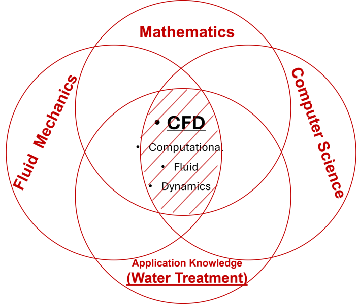
Figure 2: Conceptual diagram illustrating how Computational Fluid Dynamics (CFD) lies at the intersection of four knowledge areas: fluid mechanics, numerical methods, computer science, and application-specific engineering.

Defining the scope and level of detail

Establishing the correct scope of a CFD study is a critical first step. Engineers must determine whether the situation calls for a steady-state analysis or if transient simulation is necessary to capture time-dependent behaviour. They must also assess the nature of the tank system—whether it operates in a flow-through mode or as a closed system—and decide whether a single-phase (e.g. liquid-only) model is sufficient or if a more complex multiphase approach is warranted. Once the scope is established, it is important to identify which geometric features must be retained in the model to ensure accuracy, and which can be excluded to maintain computational feasibility. This step requires careful judgment. Excessive simplification can lead to misleading conclusions, while overly detailed models may become computationally unmanageable.

Rheology and suspended solids

Rheological properties and suspended solids play a crucial role in mixing systems. In many simulations, a homogeneous distribution of suspended solids is assumed, and fluid behaviour is modelled as either Newtonian or non-Newtonian, depending on concentration and particle characteristics. Some suspensions, such as silica-based mixtures, behave as Newtonian fluids even at high concentrations, whereas others, like polymer suspensions, exhibit non-Newtonian behaviour even at low concentrations. When rheological data is not readily available, laboratory analysis using a rheometer, preferably by a laboratory experienced with samples from relevant applications is recommended. This is particularly true for fibrous samples, which can introduce significant uncertainty in measurements. In existing installations, it is usually possible to obtain representative samples for rheological testing. In contrast, for new installations where samples are not yet available, industry expertise is essential to estimate realistic fluid behavioΒur based on prior knowledge.

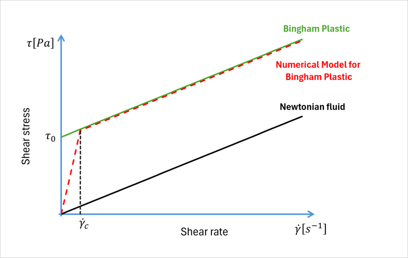
Figure 3: Example rheology diagram illustrating the relationship between shear stress and shear rate, highlighting differences between Newtonian and non-Newtonian fluid behaviour relevant to mixing applications.

When to use multiphase modelling

In scenarios involving inhomogeneous states, multiphase modelling becomes necessary. For example, in biological phosphorus removal processes, multiphase modelling is essential since sediment layers develop when mixing is lowered or deactivated, resulting in the intended or unintended formation of sludge blankets. The need to compute re-homogenization times also calls for multiphase modelling. In aerobic processes, the presence of air bubbles from aeration systems can also significantly affect mixing dynamics, necessitating a multiphase approach. These models are more complex and require additional computational resources, along with detailed and accurate input data.

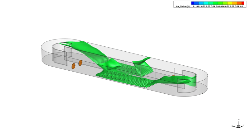
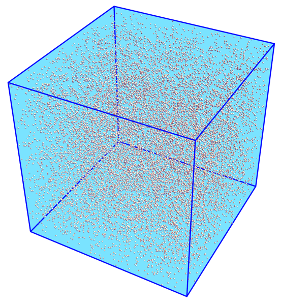
Figure 4: Multiphase CFD examples: (left) simulation of an oxidation ditch showing air plume development, and (right) visualization of air bubble dispersion in a cubic meter of water.

The computational mesh

After gathering all necessary input data, including an accurate 3-dimensional geometry, and selecting appropriate models, the next step is generating the computational mesh. This mesh forms the foundation for solving the discretised equations that govern fluid flow—a reformulation of the governing equations into a format that computers can solve. As previously mentioned, geometrical simplifications are often necessary to manage the level of detail in the model. These simplifications directly influence the mesh size—defined by the number of cells into which the domain is divided—and must be approached with careful consideration. The experience of the CFD engineer is essential in making sound judgments regarding these trade-offs.

The simulation is then run on high-performance computing infrastructure, typically on Linux-based clusters equipped with fast interconnects to support scalability and efficient resource usage. The size of the computational mesh can range from a few million to several hundred million cells, and simulation run times vary accordingly—from a few hours to several days or even weeks. The time required increases not only with mesh size but also with the complexity of the chosen models.

Figure 5: Example of a computational mesh generated for a submersible mixer CFD study, showing domain discretization into millions of cells used to resolve flow dynamics.

Assessing the quality of CFD studies

For those unfamiliar with CFD, evaluating the quality of a simulation can be challenging. Poorly executed simulations may yield inaccurate or misleading results, leading to suboptimal designs or even exacerbating existing problems. One way to mitigate this risk is to include quality specifications in the documentation accompanying any request for simulation. This helps set clear expectations and ensures that the CFD analysis meets the necessary standards. Low-quality CFD can have serious consequences, including waste of resources, ineffective or inefficient mixing, and long-term operational issues.

Postprocessing and interpretation

Once a simulation is complete and has reached convergence, the results must be carefully analysed. This stage is arguably the most subjective, requiring a high level of expertise and extensive experience in the field. Collaborating with an application engineer—even one without specific CFD expertise—can be highly beneficial. The deep understanding of the application and process can offer valuable insights, product-specific knowledge, and practical experience that help identify potential issues and avoid misinterpretations.

Even at this stage, collaboration between the CFD specialist and an experienced application engineer remains essential. It fosters quality, reduces the risk of errors, and ensures more accurate and meaningful interpretation of the results.

There are various approaches to result interpretation, ranging from global metrics such as bulk velocity, mixing homogeneity, or oxygen transfer rate, to more localized analyses using scalar and vector visualizations. Flow velocity is commonly examined through streamlines, iso-surfaces, and cross-sectional slices of the tank. The aim is often to identify areas of low velocity that may indicate stagnation and poor local mixing. Other parameters, such as air volume fraction, are visualized to assess aeration efficiency and to evaluate the risk of unwanted air entrainment, particularly near mixers or into adjacent zones. If suspended solids are included in the simulation, their concentration can also be plotted to identify sedimentation zones and evaluate overall mixing effectiveness.

In single-phase simulations where solids are not explicitly modelled, sedimentation risk can be assessed by calculating the bottom shear stress and comparing it with known re-suspension thresholds. Turbulence levels may also be evaluated to gain insight into the intensity and distribution of mixing forces throughout the tank. 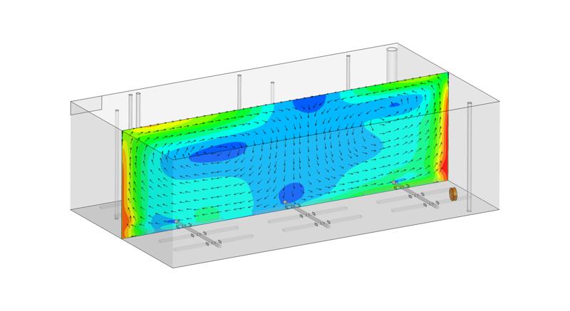Figure 6: Example CFD velocity plot with arrows indicating flow direction and colour contours representing velocity magnitude, used to identify circulation patterns and potential stagnation zones.

Mixing design and mixer placement

During the early design phase, total thrust requirements are typically estimated using simplified, low-dimensional tools. These tools are well-calibrated and generally reliable for sizing mixers—especially for standard applications and relatively simple tank geometries with few internal obstacles. However, they provide no guidance on optimal mixer placement within a specific tank configuration. This is rather drafted by an experienced application engineer.

Even when overall thrust is sufficient, certain tank geometries may create difficult-to-reach areas, reducing mixing effectiveness. This is where CFD offers a decisive advantage. By accounting for the specific characteristics of a given tank, CFD can identify areas where standard design recommendations fall short and help optimize mixer placement. An initial CFD simulation can highlight potential issues, which can then be addressed through design modifications and retested in follow-up simulations. This iterative process enables the development of a robust, efficient, and optimized mixing strategy tailored to the unique geometry and process conditions of each installation.

Troubleshooting

CFD is not only a powerful tool during the design phase—it also plays a crucial role in diagnosing and resolving issues in existing mixer installations. In wastewater treatment plants and other industrial processes, it’s not uncommon for certain functions to underperform, even in well-established systems. These issues may manifest as reduced processing capacity, increased retention times, the formation of undesirable by-products or emissions, or excessive wear and tear on equipment such as mixers, aeration systems, or auxiliary machinery within the tank.

Pinpointing the root cause of such problems can be challenging, especially when the symptoms are subtle or arise gradually. In many cases, the underlying issue is hydrodynamic in nature—stemming from poor flow distribution, dead zones, short-circuiting, or inadequate turbulence levels. Traditional diagnostic methods, such as empirical testing or trial-and-error adjustments, can be time-consuming, expensive, and inconclusive.

This is where CFD truly excels. By creating a detailed, virtual model of the tank, CFD enables engineers to visualize and analyse flow patterns, velocity fields, shear rates, and mixing efficiencies in real-time. This insight can reveal hidden inefficiencies or problematic zones that would be difficult or impossible to detect through direct observation or physical testing.

Moreover, CFD offers a safe and cost-effective environment to test proposed solutions before any physical changes are implemented. Engineers can evaluate the impact of repositioning mixers, altering thrust or blade angles, adding baffles, or adjusting operational parameters—all within the digital model. This iterative testing accelerates troubleshooting efforts and supports data-driven decision-making, ultimately leading to faster resolutions and improved plant performance.

Conclusion

Over the past few decades, Computational Fluid Dynamics (CFD) has matured into a powerful and indispensable tool, revolutionizing the way engineers design and analyse submersible mixer systems. By providing detailed, visual insights into fluid flow and mixing behaviour, CFD enables more informed engineering decisions while significantly reducing reliance on costly and time-intensive physical testing.

The effectiveness of CFD, however, hinges on several key factors: the quality and accuracy of input data, the selection of appropriate modelling approaches, and the expertise applied in interpreting results. When simulations are guided by comprehensive specification documentation and executed with care and precision, CFD can deliver substantial benefits.

These include optimized mixer performance, enhanced energy efficiency, increased system reliability, and the ability to identify and resolve operational challenges in both new and existing installations. Across a wide range of industrial and municipal applications, CFD continues to prove its value as a strategic asset in the development and improvement of modern mixing solutions.